
Nicholas Gunther
Co-Founder and Chief Solutions Officer
In Part I of the series on “Inside Agency MBS Q422: What Happened and How Money was Made,” we shared Rule 1 (a screening rule) that, had it been applied in Q422, would have helped investors to construct a portfolio to perform well in a range of potential future markets and rates. While Rule 1 is simple, the article shows it's also robust because it’s not making investors make bets on a particular future.
Now, things are about to get more interesting in Part II, where we’ll reveal two additional rules to tell the story of how money was made with the rules in place.
Rule 2: Quartile Intersection
The following two Rules are based on both scenarios described in Part I: the static scenario that didn’t happen and the market scenario that did. We first investigate perhaps the most straightforward approach to realizing outperformance in both scenarios: Rule 2 selects pools at the intersection of both the top predicted quartiles, which are known in advance for each scenario. To reduce the hindsight bias from including the market scenario, we use our knowledge of the (ex-ante) convexity risk from the highest coupons (see ) and also reject coupons over 4.5%.
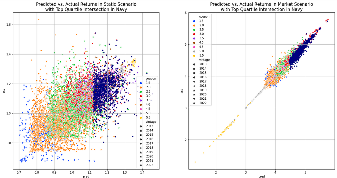
Figure 1: Rule 2 in Static and Market Scenarios
Outperformance Achieved
Because Infima’s CPR predictions, and thus return predictions, are so accurate, the 1,100 pools selected by Rule 2 in the intersection (shown larger and in navy blue in Figure 1) of the top predicted quartiles in the two scenarios above outperformed the other large pools on an actual basis, by 4.76 to 4.16% quarterly, a difference of 60 quarterly bps, in the right-hand market scenario in Figure 1, and a difference over 11 quarterly bps in the left-hand static scenario of Figure 1. The substantially increased outperformance of Rule 2 over Rule 1 in the market scenario (30 quarterly bps) is attributable to considering two scenarios, one of which was realized, showing the continuing benefit of human insight and skill.
Outperformance Analysis
Figure 2 shows that Rule 2 selected pools with higher OAS, lower duration and less (negative) convexity, while Figure 3 shows those selected pools were concentrated in 2.5 – 3.5% coupons and 2019-2020 vintages. The higher OAS and lack of negative convexity provided the selected pools with a robust return across a range of rate environments; their coupon concentration avoided both the deepest discount and the risk of becoming premium collateral in lower-price environments. Note the similar profile to that of Rule 1.
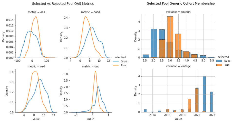
Figure 2: OAS Metric Comparison Selected vs. Rejected; Figure 3: Selected vs. Reject by Coupon & Vintage
Rule 3: Efficient Frontier
Rule 3, the last rule considered in depth, combines the two scenarios by using the associated predicted returns as the metrics in a two-metric Efficient Frontier.4 While somewhat more complex than the simple intersection of Rule 2, Rule 3 lets clients select pools based on their subjective assessment of the full range of relative scenario likelihoods without exact numerical weights, as described in greater detail below.
Even considering both scenarios, at the time of portfolio formation in October 2022, an investor can only access predicted CPRs. Figure 8 is, therefore, the basis for an investor’s ex-ante investment decision; it shows the Efficient Frontier (EF) for predicted pool returns in the static and market scenarios based on Infima’s predicted CPRs. Note that the pools on the dotted red line segment(s) in the upper right of Figure 4 have the optimal combinations of returns in both scenarios, and pools near that segment are nearly optimal. Every point on or inside the boundary (the thin closed black line containing the EF), whether or not corresponding to an actual pool, can be constructed as a long-only portfolio in the displayed MBS pools, typically in many ways. Thus, investors can position their long MBS investments anywhere on or inside that boundary but not outside the boundary without taking short positions.
No pool on the EF is best in both scenarios simultaneously; for any pair of pools, each pool is better in one scenario but worse in the other. Accordingly, an investor who believes the static scenario is more likely would, based on Figure 4, prefer pool CA6317 to AS8085, while an investor who thought the reverse would choose the latter pool. The distance to the EF provides a single metric that measures how close to optimal a pool is in light of both scenarios. Investors can use this metric to select optimal or nearly optimal pools, considering both scenarios at once while “tilting” the selection to fit an investor’s individual beliefs about the scenarios’ relative likelihoods without assigning specific scenario weights.
Figure 5 shows the EF for (1) predicted static returns on the x-axis and (2) actual market returns based on realized CPRs on the y-axis. Given Infima’s exceptional prepayment prediction accuracy, the graphs in Figures 4 & 5 are extremely close. As a result, the pools nearest the two EFs are also very similar. However, requiring as it does the realized CPRs, Figure 5 EF is known only with the benefit of hindsight. Nonetheless, as Table 1 shows, the pools closest to the realized market EF (see the column dist2boundary_predreal) in Figure 5 are very similar to those closest to the predicted market EF (see the column dist2boundary_predpred) in Figure 4, and - interestingly - also those in the top quartile intersection, with which they share similar coupon and vintage concentrations. Figure 6 shows these two sets of pools also share similar OAS metrics; the pools selected by the EF method have higher than average OAS but avoid the highest OAS and the corresponding, highest coupons.
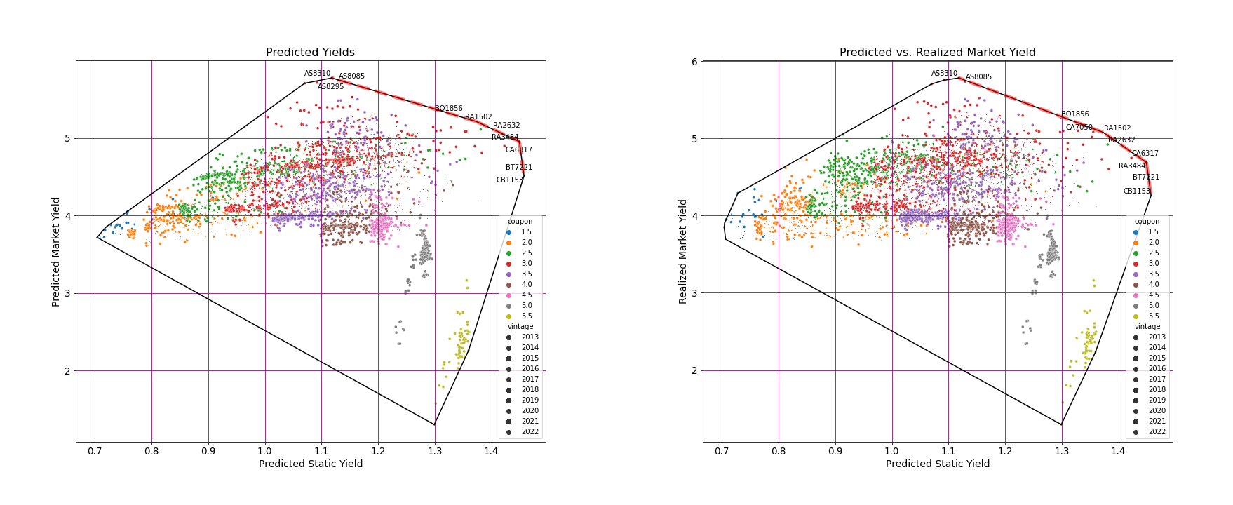
Figure 4: Efficient Frontier for Predicted Formula and Market Returns; Figure 5: Efficient Frontier for Predicted Formula and Realized Market Returns
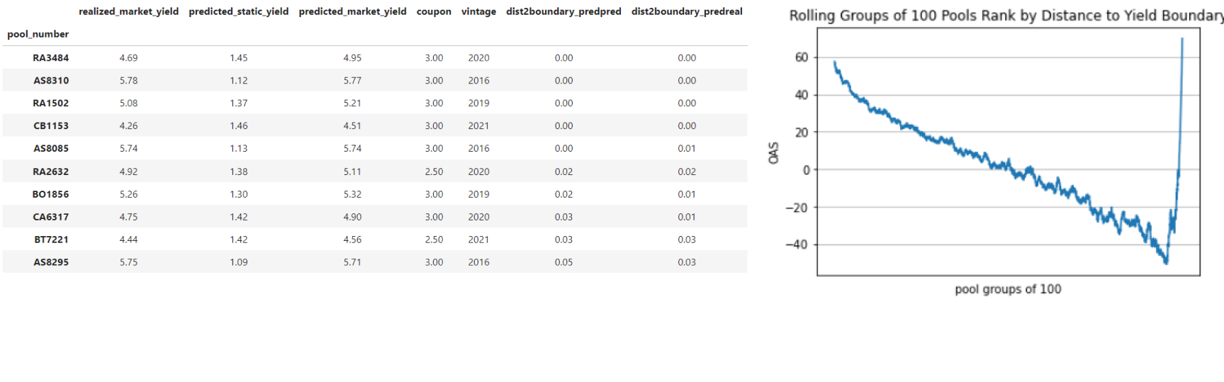
Table 1: Pools Returns, with Distance to Realized Market EF; Figure 6: OAS vs. Distance to Efficient Frontier
Modeling outperformance
A very different but conventional approach is to model outperformance directly or via classification. To take one example of a direct model, consider an investor with strong quantitative beliefs about the likelihood of two or more scenarios expressed as specific weights. Such an investor can use those weights to combine the predicted scenario pool returns into a single series of composite predicted pool returns that can be optimized directly. Alternatively, the realized pool returns can be treated as the dependent variable in a regression model, with the Infima’s predicted returns in multiple scenarios, together with OAS metrics and/or other features, as explanatory variables.
For another example, a classification model of the pool quartile intersection using Infima’s return predictions, OAS metrics, and pool features can predict whether a pool is likely to be in the top predicted-quartile intersection. Such a model can then learn what makes a pool likely to be among the top performers simultaneously in multiple environments.
Summary
Investors can realize outperformance by selecting pools predicted by Infima to outperform over an appropriate range of scenarios, such as (1) scenario quartile intersections and (2) scenario Efficient Frontiers, as detailed above. Stay tuned for Part III, when we apply some of the same techniques to position for future expected outperformance.
